

In machine learning, Feature selection is the process of choosing variables that are useful in predicting the response (Y).
It is considered a good practice to identify which features are important when building predictive models.
In this post, you will see how to implement 10 powerful feature selection approaches in R.
2. Variable Importance from Machine Learning Algorithms
3. Lasso Regression 4. Step wise Forward and Backward Selection 5. Relative Importance from Linear Regression 6. Recursive Feature Elimination (RFE) 7. Genetic Algorithm 8. Simulated Annealing 9. Information Value and Weights of Evidence 10. DALEX Package Conclusion
Introduction
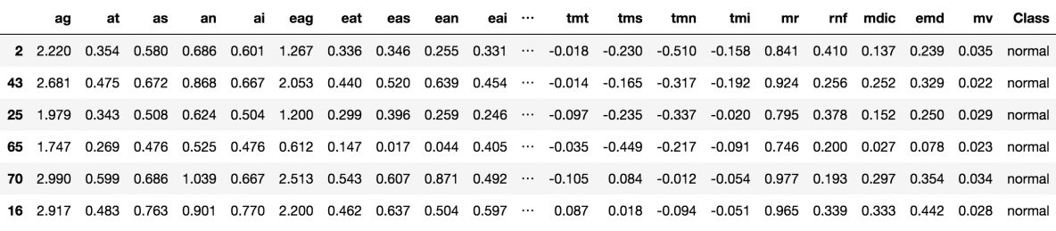
In real-world datasets, it is fairly common to have columns that are nothing but noise. You are better off getting rid of such variables because of the memory space they occupy, the time and the computational resources it is going to cost, especially in large datasets. Sometimes, you have a variable that makes business sense, but you are not sure if it actually helps in predicting the Y. You also need to consider the fact that, a feature that could be useful in one ML algorithm (say a decision tree) may go underrepresented or unused by another (like a regression model). Having said that, it is still possible that a variable that shows poor signs of helping to explain the response variable (Y), can turn out to be significantly useful in the presence of (or combination with) other predictors. What I mean by that is, a variable might have a low correlation value of (~0.2) with Y. But in the presence of other variables, it can help to explain certain patterns/phenomenon that other variables can’t explain. In such cases, it can be hard to make a call whether to include or exclude such variables. The strategies we are about to discuss can help fix such problems. Not only that, it will also help understand if a particular variable is important or not and how much it is contributing to the model An important caveat. It is always best to have variables that have sound business logic backing the inclusion of a variable and rely solely on variable importance metrics. Alright. Let’s load up the 'Glaucoma' dataset where the goal is to predict if a patient has Glaucoma or not based on 63 different physiological measurements. You can directly run the codes or download the dataset here. A lot of interesting examples ahead. Let’s get started.
# Load Packages and prepare dataset
library(TH.data)
library(caret)
data("GlaucomaM", package = "TH.data")
trainData <- GlaucomaM
head(trainData)
1. Boruta
Boruta is a feature ranking and selection algorithm based on random forests algorithm. The advantage with Boruta is that it clearly decides if a variable is important or not and helps to select variables that are statistically significant. Besides, you can adjust the strictness of the algorithm by adjusting the p values that defaults to 0.01 and the maxRuns. maxRuns is the number of times the algorithm is run. The higher the maxRuns the more selective you get in picking the variables. The default value is 100. In the process of deciding if a feature is important or not, some features may be marked by Boruta as 'Tentative'. Sometimes increasing the maxRuns can help resolve the 'Tentativeness' of the feature. Lets see an example based on the Glaucoma dataset from TH.data package that I created earlier.
# install.packages('Boruta')
library(Boruta)
The boruta function uses a formula interface just like most predictive modeling functions. So the first argument to boruta() is the formula with the response variable on the left and all the predictors on the right. By placing a dot, all the variables in trainData other than Class will be included in the model. The doTrace argument controls the amount of output printed to the console. Higher the value, more the log details you get. So save space I have set it to 0, but try setting it to 1 and 2 if you are running the code. Finally the output is stored in boruta_output.
# Perform Boruta search
boruta_output <- Boruta(Class ~ ., data=na.omit(trainData), doTrace=0)
Let’s see what the boruta_output contains.
names(boruta_output)
- ‘finalDecision’
- ‘ImpHistory’
- ‘pValue’
- ‘maxRuns’
- ‘light’
- ‘mcAdj’
- ‘timeTaken’
- ‘roughfixed’
- ‘call’
- ‘impSource’
# Get significant variables including tentatives
boruta_signif <- getSelectedAttributes(boruta_output, withTentative = TRUE)
print(boruta_signif)
 [1] "as"   "ean"  "abrg" "abrs" "abrn" "abri" "hic"  "mhcg" "mhcn" "mhci"
[11] "phcg" "phcn" "phci" "hvc"  "vbss" "vbsn" "vbsi" "vasg" "vass" "vasi"
[21] "vbrg" "vbrs" "vbrn" "vbri" "varg" "vart" "vars" "varn" "vari" "mdn"
[31] "tmg"  "tmt"  "tms"  "tmn"  "tmi"  "rnf"  "mdic" "emd"
If you are not sure about the tentative variables being selected for granted, you can choose a TentativeRoughFix on boruta_output.
# Do a tentative rough fix
roughFixMod <- TentativeRoughFix(boruta_output)
boruta_signif <- getSelectedAttributes(roughFixMod)
print(boruta_signif)
 [1] "abrg" "abrs" "abrn" "abri" "hic"  "mhcg" "mhcn" "mhci" "phcg" "phcn"
[11] "phci" "hvc"  "vbsn" "vbsi" "vasg" "vbrg" "vbrs" "vbrn" "vbri" "varg"
[21] "vart" "vars" "varn" "vari" "tmg"  "tms"  "tmi"  "rnf"  "mdic" "emd"
There you go. Boruta has decided on the ‘Tentative’ variables on our behalf. Let’s find out the importance scores of these variables.
# Variable Importance Scores
imps <- attStats(roughFixMod)
imps2 = imps[imps$decision != 'Rejected', c('meanImp', 'decision')]
head(imps2[order(-imps2$meanImp), ])  # descending sort
| meanImp | decision | |
|---|---|---|
| varg | 10.279747 | Confirmed |
| vari | 10.245936 | Confirmed |
| tmi | 9.067300 | Confirmed |
| vars | 8.690654 | Confirmed |
| hic | 8.324252 | Confirmed |
| varn | 7.327045 | Confirmed |
Let’s plot it to see the importances of these variables.
# Plot variable importance
plot(boruta_output, cex.axis=.7, las=2, xlab="", main="Variable Importance")
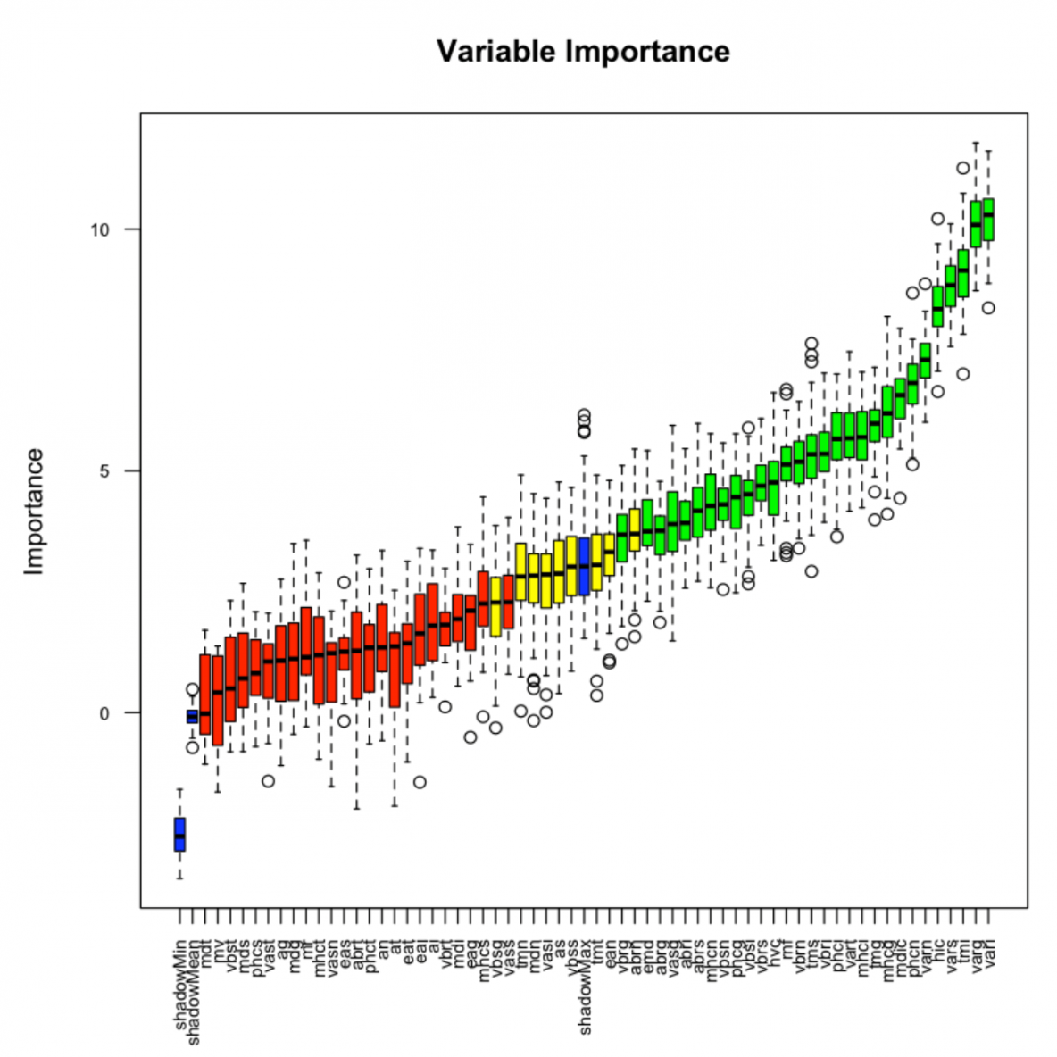
This plot reveals the importance of each of the features. The columns in green are ‘confirmed’ and the ones in red are not. There are couple of blue bars representing ShadowMax and ShadowMin. They are not actual features, but are used by the boruta algorithm to decide if a variable is important or not.

2. Variable Importance from Machine Learning Algorithms
Another way to look at feature selection is to consider variables most used by various ML algorithms the most to be important. Depending on how the machine learning algorithm learns the relationship between X’s and Y, different machine learning algorithms may possibly end up using different variables (but mostly common vars) to various degrees. What I mean by that is, the variables that proved useful in a tree-based algorithm like rpart, can turn out to be less useful in a regression-based model. So all variables need not be equally useful to all algorithms. So how do we find the variable importance for a given ML algo?
train()the desired model using the caret package.- Then, use
varImp()to determine the feature importances.
You may want to try out multiple algorithms, to get a feel of the usefulness of the features across algos.
# Train an rpart model and compute variable importance.
library(caret)
set.seed(100)
rPartMod <- train(Class ~ ., data=trainData, method="rpart")
rpartImp <- varImp(rPartMod)
print(rpartImp)
rpart variable importance

  only 20 most important variables shown (out of 62)

     Overall
varg  100.00
vari   93.19
vars   85.20
varn   76.86
tmi    72.31
vbss    0.00
eai     0.00
tmg     0.00
tmt     0.00
vbst    0.00
vasg    0.00
at      0.00
abrg    0.00
vbsg    0.00
eag     0.00
phcs    0.00
abrs    0.00
mdic    0.00
abrt    0.00
ean     0.00
Only 5 of the 63 features was used by rpart and if you look closely, the 5 variables used here are in the top 6 that boruta selected. Let’s do one more: the variable importances from Regularized Random Forest (RRF) algorithm.
# Train an RRF model and compute variable importance.
set.seed(100)
rrfMod <- train(Class ~ ., data=trainData, method="RRF")
rrfImp <- varImp(rrfMod, scale=F)
rrfImp
RRF variable importance

  only 20 most important variables shown (out of 62)

     Overall
varg 24.0013
vari 18.5349
vars  6.0483
tmi   3.8699
hic   3.3926
mhci  3.1856
mhcg  3.0383
mv    2.1570
hvc   2.1357
phci  1.8830
vasg  1.8570
tms   1.5705
phcn  1.4475
phct  1.4473
vass  1.3097
tmt   1.2485
phcg  1.1992
mdn   1.1737
tmg   1.0988
abrs  0.9537
plot(rrfImp, top = 20, main='Variable Importance')
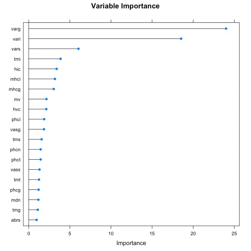
The topmost important variables are pretty much from the top tier of Boruta‘s selections. Some of the other algorithms available in train() that you can use to compute varImp are the following: ada, AdaBag, AdaBoost.M1, adaboost, bagEarth, bagEarthGCV, bagFDA, bagFDAGCV, bartMachine, blasso, BstLm, bstSm, C5.0, C5.0Cost, C5.0Rules, C5.0Tree, cforest, chaid, ctree, ctree2, cubist, deepboost, earth, enet, evtree, extraTrees, fda, gamboost, gbm_h2o, gbm, gcvEarth, glmnet_h2o, glmnet, glmStepAIC, J48, JRip, lars, lars2, lasso, LMT, LogitBoost, M5, M5Rules, msaenet, nodeHarvest, OneR, ordinalNet, ORFlog, ORFpls, ORFridge, ORFsvm, pam, parRF, PART, penalized, PenalizedLDA, qrf, ranger, Rborist, relaxo, rf, rFerns, rfRules, rotationForest, rotationForestCp, rpart, rpart1SE, rpart2, rpartCost, rpartScore, rqlasso, rqnc, RRF, RRFglobal, sdwd, smda, sparseLDA, spikeslab, wsrf, xgbLinear, xgbTree.
3. Lasso Regression
Least Absolute Shrinkage and Selection Operator (LASSO) regression is a type of regularization method that penalizes with L1-norm. It basically imposes a cost to having large weights (value of coefficients). And its called L1 regularization, because the cost added, is proportional to the absolute value of weight coefficients. As a result, in the process of shrinking the coefficients, it eventually reduces the coefficients of certain unwanted features all the to zero. That is, it removes the unneeded variables altogether. So effectively, LASSO regression can be considered as a variable selection technique as well.
library(glmnet)
trainData <- read.csv('https://raw.githubusercontent.com/selva86/datasets/master/GlaucomaM.csv')

x <- as.matrix(trainData[,-63]) # all X vars
y <- as.double(as.matrix(ifelse(trainData[, 63]=='normal', 0, 1))) # Only Class

# Fit the LASSO model (Lasso: Alpha = 1)
set.seed(100)
cv.lasso <- cv.glmnet(x, y, family='binomial', alpha=1, parallel=TRUE, standardize=TRUE, type.measure='auc')

# Results
plot(cv.lasso)
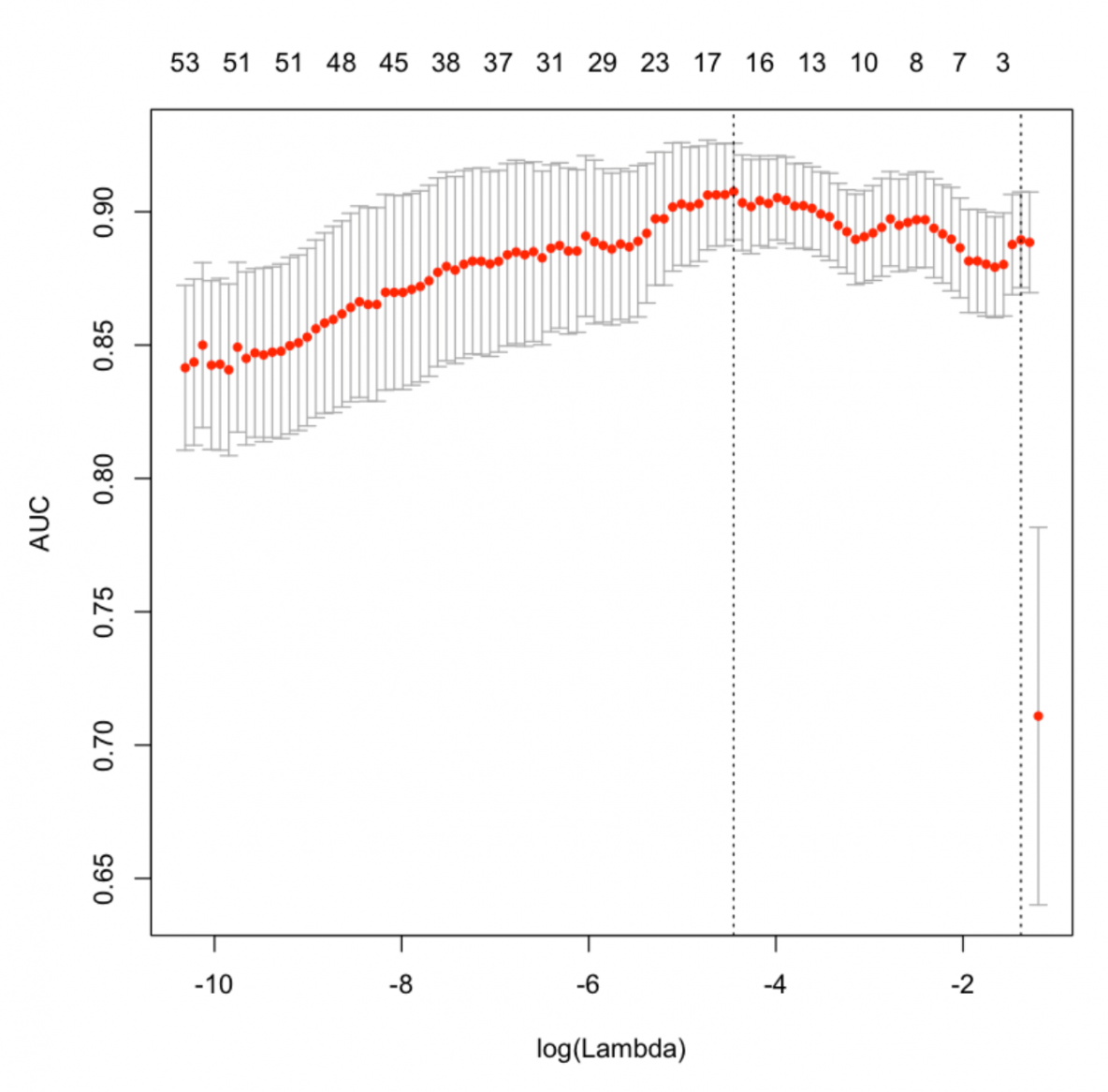
Let’s see how to interpret this plot. The X axis of the plot is the log of lambda. That means when it is 2 here, the lambda value is actually 100. The numbers at the top of the plot show how many predictors were included in the model. The position of red dots along the Y-axis tells what AUC we got when you include as many variables shown on the top x-axis. You can also see two dashed vertical lines. The first one on the left points to the lambda with the lowest mean squared error. The one on the right point to the number of variables with the highest deviance within 1 standard deviation. The best lambda value is stored inside 'cv.lasso$lambda.min'.
# plot(cv.lasso$glmnet.fit, xvar="lambda", label=TRUE)
cat('Min Lambda: ', cv.lasso$lambda.min, '\n 1Sd Lambda: ', cv.lasso$lambda.1se)
df_coef <- round(as.matrix(coef(cv.lasso, s=cv.lasso$lambda.min)), 2)

# See all contributing variables
df_coef[df_coef[, 1] != 0, ]
Min Lambda:  0.01166507
 1Sd Lambda:  0.2513163

Min Lambda:  0.01166507
1Sd Lambda:  0.2513163

(Intercept) 3.65
at         -0.17
as         -2.05
eat        -0.53
mhci        6.22
phcs       -0.83
phci        6.03
hvc        -4.15
vass       -23.72
vbrn       -0.26
vars       -25.86
mdt        -2.34
mds         0.5
mdn         0.83
mdi         0.3
tmg         0.01
tms         3.02
tmi         2.65
mv          4.94
The above output shows what variables LASSO considered important. A high positive or low negative implies more important is that variable.
4. Step wise Forward and Backward Selection
Stepwise regression can be used to select features if the Y variable is a numeric variable. It is particularly used in selecting best linear regression models. It searches for the best possible regression model by iteratively selecting and dropping variables to arrive at a model with the lowest possible AIC. It can be implemented using the step() function and you need to provide it with a lower model, which is the base model from which it won’t remove any features and an upper model, which is a full model that has all possible features you want to have. Our case is not so complicated (< 20 vars), so lets just do a simple stepwise in 'both' directions. I will use the ozone dataset for this where the objective is to predict the 'ozone_reading' based on other weather related observations.
# Load data
trainData <- read.csv("http://rstatistics.net/wp-content/uploads/2015/09/ozone1.csv", stringsAsFactors=F)
print(head(trainData))
  Month Day_of_month Day_of_week ozone_reading pressure_height Wind_speed
1     1            1           4             3            5480          8
2     1            2           5             3            5660          6
3     1            3           6             3            5710          4
4     1            4           7             5            5700          3
5     1            5           1             5            5760          3
6     1            6           2             6            5720          4

  Humidity Temperature_Sandburg Temperature_ElMonte Inversion_base_height
1 20.00000             40.53473            39.77461              5000.000
2 40.96306             38.00000            46.74935              4108.904
3 28.00000             40.00000            49.49278              2693.000
4 37.00000             45.00000            52.29403               590.000
5 51.00000             54.00000            45.32000              1450.000
6 69.00000             35.00000            49.64000              1568.000

  Pressure_gradient Inversion_temperature Visibility
1               -15              30.56000        200
2               -14              48.02557        300
3               -25              47.66000        250
4               -24              55.04000        100
5                25              57.02000         60
6                15              53.78000         60
The data is ready. Let’s perform the stepwise.
# Step 1: Define base intercept only model
base.mod <- lm(ozone_reading ~ 1 , data=trainData)

# Step 2: Full model with all predictors
all.mod <- lm(ozone_reading ~ . , data= trainData)

# Step 3: Perform step-wise algorithm. direction='both' implies both forward and backward stepwise
stepMod <- step(base.mod, scope = list(lower = base.mod, upper = all.mod), direction = "both", trace = 0, steps = 1000)

# Step 4: Get the shortlisted variable.
shortlistedVars <- names(unlist(stepMod[[1]]))
shortlistedVars <- shortlistedVars[!shortlistedVars %in% "(Intercept)"] # remove intercept

# Show
print(shortlistedVars)
[1] "Temperature_Sandburg"  "Humidity"              "Temperature_ElMonte"
[4] "Month"                 "pressure_height"       "Inversion_base_height"
The selected model has the above 6 features in it. But if you have too many features (> 100) in training data, then it might be a good idea to split the dataset into chunks of 10 variables each with Y as mandatory in each dataset. Loop through all the chunks and collect the best features. We are doing it this way because some variables that came as important in a training data with fewer features may not show up in a linear reg model built on lots of features. Finally, from a pool of shortlisted features (from small chunk models), run a full stepwise model to get the final set of selected features. You can take this as a learning assignment to be solved within 20 minutes.
5. Relative Importance from Linear Regression
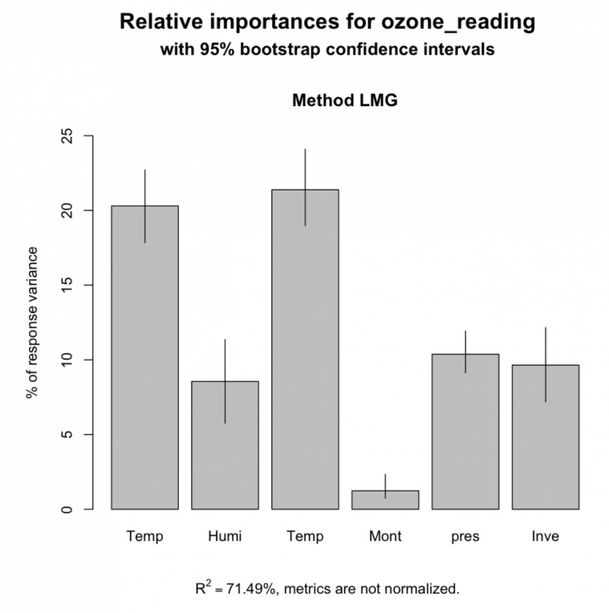
This technique is specific to linear regression models. Relative importance can be used to assess which variables contributed how much in explaining the linear model’s R-squared value. So, if you sum up the produced importances, it will add up to the model’s R-sq value. In essence, it is not directly a feature selection method, because you have already provided the features that go in the model. But after building the model, the relaimpo can provide a sense of how important each feature is in contributing to the R-sq, or in other words, in ‘explaining the Y variable’. So, how to calculate relative importance? It is implemented in the relaimpo package. Basically, you build a linear regression model and pass that as the main argument to calc.relimp(). relaimpo has multiple options to compute the relative importance, but the recommended method is to use type='lmg', as I have done below.
# install.packages('relaimpo')
library(relaimpo)

# Build linear regression model
model_formula = ozone_reading ~ Temperature_Sandburg + Humidity + Temperature_ElMonte + Month + pressure_height + Inversion_base_height
lmMod <- lm(model_formula, data=trainData)

# calculate relative importance
relImportance <- calc.relimp(lmMod, type = "lmg", rela = F)

# Sort
cat('Relative Importances: \n')
sort(round(relImportance$lmg, 3), decreasing=TRUE)
Relative Importances:
Temperature_ElMonte    0.214
Temperature_Sandburg   0.203
pressure_height        0.104
Inversion_base_height  0.096
Humidity               0.086
Month                  0.012
Additionally, you can use bootstrapping (using boot.relimp) to compute the confidence intervals of the produced relative importances.
bootsub <- boot.relimp(ozone_reading ~ Temperature_Sandburg + Humidity + Temperature_ElMonte + Month + pressure_height + Inversion_base_height, data=trainData,
                       b = 1000, type = 'lmg', rank = TRUE, diff = TRUE)

plot(booteval.relimp(bootsub, level=.95))
6. Recursive Feature Elimination (RFE)
Recursive feature elimnation (rfe) offers a rigorous way to determine the important variables before you even feed them into a ML algo. It can be implemented using the rfe() from caret package. The rfe() also takes two important parameters.
- sizes
- rfeControl
So, what does sizes and rfeControl represent? The sizes determines the number of most important features the rfe should iterate. Below, I have set the size as 1 to 5, 10, 15 and 18. Secondly, the rfeControl parameter receives the output of the rfeControl(). You can set what type of variable evaluation algorithm must be used. Here, I have used random forests based rfFuncs. The method='repeatedCV' means it will do a repeated k-Fold cross validation with repeats=5. Once complete, you get the accuracy and kappa for each model size you provided. The final selected model subset size is marked with a * in the rightmost selected column.
str(trainData)
'data.frame':    366 obs. of  13 variables:
 $ Month                : int  1 1 1 1 1 1 1 1 1 1 ...
 $ Day_of_month         : int  1 2 3 4 5 6 7 8 9 10 ...
 $ Day_of_week          : int  4 5 6 7 1 2 3 4 5 6 ...
 $ ozone_reading        : num  3 3 3 5 5 6 4 4 6 7 ...
 $ pressure_height      : num  5480 5660 5710 5700 5760 5720 5790 5790 5700 5700 ...
 $ Wind_speed           : int  8 6 4 3 3 4 6 3 3 3 ...
 $ Humidity             : num  20 41 28 37 51 ...
 $ Temperature_Sandburg : num  40.5 38 40 45 54 ...
 $ Temperature_ElMonte  : num  39.8 46.7 49.5 52.3 45.3 ...
 $ Inversion_base_height: num  5000 4109 2693 590 1450 ...
 $ Pressure_gradient    : num  -15 -14 -25 -24 25 15 -33 -28 23 -2 ...
 $ Inversion_temperature: num  30.6 48 47.7 55 57 ...
 $ Visibility           : int  200 300 250 100 60 60 100 250 120 120 ...
set.seed(100)
options(warn=-1)

subsets <- c(1:5, 10, 15, 18)

ctrl <- rfeControl(functions = rfFuncs,
                   method = "repeatedcv",
                   repeats = 5,
                   verbose = FALSE)

lmProfile <- rfe(x=trainData[, c(1:3, 5:13)], y=trainData$ozone_reading,
                 sizes = subsets,
                 rfeControl = ctrl)

lmProfile
Recursive feature selection

Outer resampling method: Cross-Validated (10 fold, repeated 5 times)

Resampling performance over subset size:

 Variables  RMSE Rsquared   MAE RMSESD RsquaredSD  MAESD Selected
         1 5.222   0.5794 4.008 0.9757    0.15034 0.7879
         2 3.971   0.7518 3.067 0.4614    0.07149 0.3276
         3 3.944   0.7553 3.054 0.4675    0.06523 0.3708
         4 3.924   0.7583 3.026 0.5132    0.06640 0.4163
         5 3.880   0.7633 2.950 0.5525    0.07021 0.4334
        10 3.751   0.7796 2.853 0.5550    0.06791 0.4457        *
        12 3.767   0.7779 2.869 0.5511    0.06664 0.4424

The top 5 variables (out of 10):
   Temperature_ElMonte, Pressure_gradient, Temperature_Sandburg, Inversion_temperature, Humidity
So, it says, Temperature_ElMonte, Pressure_gradient, Temperature_Sandburg, Inversion_temperature, Humidity are the top 5 variables in that order. And the best model size out of the provided models sizes (in subsets) is 10. You can see all of the top 10 variables from 'lmProfile$optVariables' that was created using rfe function above.
7. Genetic Algorithm
You can perform a supervised feature selection with genetic algorithms using the gafs(). This is quite resource expensive so consider that before choosing the number of iterations (iters) and the number of repeats in gafsControl().
# Define control function
ga_ctrl <- gafsControl(functions = rfGA,  # another option is `caretGA`.
                        method = "cv",
                        repeats = 3)

# Genetic Algorithm feature selection
set.seed(100)
ga_obj <- gafs(x=trainData[, c(1:3, 5:13)],
               y=trainData[, 4],
               iters = 3,   # normally much higher (100+)
               gafsControl = ga_ctrl)

ga_obj
Genetic Algorithm Feature Selection

366 samples
12 predictors

Maximum generations: 3
Population per generation: 50
Crossover probability: 0.8
Mutation probability: 0.1
Elitism: 0

Internal performance values: RMSE, Rsquared
Subset selection driven to minimize internal RMSE

External performance values: RMSE, Rsquared, MAE
Best iteration chose by minimizing external RMSE
External resampling method: Cross-Validated (10 fold)

During resampling:
  * the top 5 selected variables (out of a possible 12):
    Month (100%), Pressure_gradient (100%), Temperature_ElMonte (100%), Visibility (90%), Inversion_temperature (80%)
  * on average, 7.5 variables were selected (min = 5, max = 10)

In the final search using the entire training set:
   * 6 features selected at iteration 3 including:
     Month, Day_of_month, Wind_speed, Temperature_ElMonte, Pressure_gradient ...
   * external performance at this iteration is

       RMSE    Rsquared         MAE
     3.6605      0.7901      2.8010
# Optimal variables
ga_obj$optVariables
- ‘Month’
- ‘Day_of_month’
- ‘Wind_speed’
- ‘Temperature_ElMonte’
- ‘Pressure_gradient’
- ‘Visibility’
So the optimal variables according to the genetic algorithms are listed above. But, I wouldn’t use it just yet because, the above variant was tuned for only 3 iterations, which is quite low. I had to set it so low to save computing time.
8. Simulated Annealing
Simulated annealing is a global search algorithm that allows a suboptimal solution to be accepted in hope that a better solution will show up eventually. It works by making small random changes to an initial solution and sees if the performance improved. The change is accepted if it improves, else it can still be accepted if the difference of performances meet an acceptance criteria. In caret it has been implemented in the safs() which accepts a control parameter that can be set using the safsControl() function. safsControl is similar to other control functions in caret (like you saw in rfe and ga), and additionally it accepts an improve parameter which is the number of iterations it should wait without improvement until the values are reset to previous iteration.
# Define control function
sa_ctrl <- safsControl(functions = rfSA,
                        method = "repeatedcv",
                        repeats = 3,
                        improve = 5) # n iterations without improvement before a reset

# Genetic Algorithm feature selection
set.seed(100)
sa_obj <- safs(x=trainData[, c(1:3, 5:13)],
               y=trainData[, 4],
               safsControl = sa_ctrl)

sa_obj
Simulated Annealing Feature Selection

366 samples
12 predictors

Maximum search iterations: 10
Restart after 5 iterations without improvement (0.2 restarts on average)

Internal performance values: RMSE, Rsquared
Subset selection driven to minimize internal RMSE

External performance values: RMSE, Rsquared, MAE
Best iteration chose by minimizing external RMSE
External resampling method: Cross-Validated (10 fold, repeated 3 times)

During resampling:
  * the top 5 selected variables (out of a possible 12):
    Temperature_ElMonte (73.3%), Inversion_temperature (63.3%), Month (60%), Day_of_week (50%), Inversion_base_height (50%)
  * on average, 6 variables were selected (min = 3, max = 8)

In the final search using the entire training set:
   * 6 features selected at iteration 10 including:
     Month, Day_of_month, Day_of_week, Wind_speed, Temperature_ElMonte ...
   * external performance at this iteration is

       RMSE    Rsquared         MAE
     4.0574      0.7382      3.0727
# Optimal variables
print(sa_obj$optVariables)
[1] "Month"               "Day_of_month"        "Day_of_week"
[4] "Wind_speed"          "Temperature_ElMonte" "Visibility"
9. Information Value and Weights of Evidence
The Information Value can be used to judge how important a given categorical variable is in explaining the binary Y variable. It goes well with logistic regression and other classification models that can model binary variables. Let’s try to find out how important the categorical variables are in predicting if an individual will earn >50k from the ‘adult.csv’ dataset. Just run the code below to import the dataset.
library(InformationValue)
inputData <- read.csv("http://rstatistics.net/wp-content/uploads/2015/09/adult.csv")
print(head(inputData))
  AGE         WORKCLASS FNLWGT  EDUCATION EDUCATIONNUM       MARITALSTATUS
1  39         State-gov  77516  Bachelors           13       Never-married
2  50  Self-emp-not-inc  83311  Bachelors           13  Married-civ-spouse
3  38           Private 215646    HS-grad            9            Divorced
4  53           Private 234721       11th            7  Married-civ-spouse
5  28           Private 338409  Bachelors           13  Married-civ-spouse
6  37           Private 284582    Masters           14  Married-civ-spouse

          OCCUPATION   RELATIONSHIP   RACE     SEX CAPITALGAIN CAPITALLOSS
1       Adm-clerical  Not-in-family  White    Male        2174           0
2    Exec-managerial        Husband  White    Male           0           0
3  Handlers-cleaners  Not-in-family  White    Male           0           0
4  Handlers-cleaners        Husband  Black    Male           0           0
5     Prof-specialty           Wife  Black  Female           0           0
6    Exec-managerial           Wife  White  Female           0           0

  HOURSPERWEEK  NATIVECOUNTRY ABOVE50K
1           40  United-States        0
2           13  United-States        0
3           40  United-States        0
4           40  United-States        0
5           40           Cuba        0
6           40  United-States        0
Alright, let’s now find the information value for the categorical variables in the inputData.
# Choose Categorical Variables to compute Info Value.
cat_vars <- c ("WORKCLASS", "EDUCATION", "MARITALSTATUS", "OCCUPATION", "RELATIONSHIP", "RACE", "SEX", "NATIVECOUNTRY")  # get all categorical variables

# Init Output
df_iv <- data.frame(VARS=cat_vars, IV=numeric(length(cat_vars)), STRENGTH=character(length(cat_vars)), stringsAsFactors = F)  # init output dataframe

# Get Information Value for each variable
for (factor_var in factor_vars){
  df_iv[df_iv$VARS == factor_var, "IV"] <- InformationValue::IV(X=inputData[, factor_var], Y=inputData$ABOVE50K)
  df_iv[df_iv$VARS == factor_var, "STRENGTH"] <- attr(InformationValue::IV(X=inputData[, factor_var], Y=inputData$ABOVE50K), "howgood")
}

# Sort
df_iv <- df_iv[order(-df_iv$IV), ]

df_iv
| VARS | IV | STRENGTH | |
|---|---|---|---|
| 5 | RELATIONSHIP | 1.53560810 | Highly Predictive |
| 3 | MARITALSTATUS | 1.33882907 | Highly Predictive |
| 4 | OCCUPATION | 0.77622839 | Highly Predictive |
| 2 | EDUCATION | 0.74105372 | Highly Predictive |
| 7 | SEX | 0.30328938 | Highly Predictive |
| 1 | WORKCLASS | 0.16338802 | Highly Predictive |
| 8 | NATIVECOUNTRY | 0.07939344 | Somewhat Predictive |
| 6 | RACE | 0.06929987 | Somewhat Predictive |
Here is what the quantum of Information Value means:
- Less than 0.02, then the predictor is not useful for modeling (separating the Goods from the Bads)
- 0.02 to 0.1, then the predictor has only a weak relationship.
- 0.1 to 0.3, then the predictor has a medium strength relationship.
- 0.3 or higher, then the predictor has a strong relationship.
That was about IV. Then what is Weight of Evidence? Weights of evidence can be useful to find out how important a given categorical variable is in explaining the ‘events’ (called ‘Goods’ in below table.)
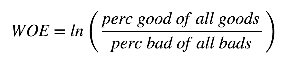
The ‘Information Value’ of the categorical variable can then be derived from the respective WOE values. IV?=?(perc good of all goods?perc bad of all bads)?*?WOE The ‘WOETable’ below given the computation in more detail.
WOETable(X=inputData[, 'WORKCLASS'], Y=inputData$ABOVE50K)
| CAT | GOODS | BADS | TOTAL | PCT_G | PCT_B | WOE | IV |
|---|---|---|---|---|---|---|---|
| ? | 191 | 1645 | 1836 | 0.0242940728 | 0.0665453074 | -1.0076506 | 0.0425744832 |
| Federal-gov | 371 | 589 | 960 | 0.0471890104 | 0.0238268608 | 0.6833475 | 0.0159644662 |
| Local-gov | 617 | 1476 | 2093 | 0.0784787586 | 0.0597087379 | 0.2733496 | 0.0051307781 |
| Never-worked | 7 | 7 | 7 | 0.0008903587 | 0.0002831715 | 1.1455716 | 0.0006955764 |
| Private | 4963 | 17733 | 22696 | 0.6312643093 | 0.7173543689 | -0.1278453 | 0.0110062102 |
| Self-emp-inc | 622 | 494 | 1116 | 0.0791147291 | 0.0199838188 | 1.3759762 | 0.0813627242 |
| Self-emp-not-inc | 724 | 1817 | 2541 | 0.0920885271 | 0.0735032362 | 0.2254209 | 0.0041895135 |
| State-gov | 353 | 945 | 1298 | 0.0448995167 | 0.0382281553 | 0.1608547 | 0.0010731201 |
| Without-pay | 14 | 14 | 14 | 0.0017807174 | 0.0005663430 | 1.1455716 | 0.0013911528 |
The total IV of a variable is the sum of IV?s of its categories.
10. DALEX Package
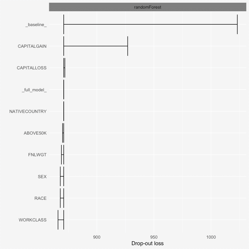
The DALEX is a powerful package that explains various things about the variables used in an ML model. For example, using the variable_dropout() function you can find out how important a variable is based on a dropout loss, that is how much loss is incurred by removing a variable from the model. Apart from this, it also has the single_variable() function that gives you an idea of how the model’s output will change by changing the values of one of the X’s in the model. It also has the single_prediction() that can decompose a single model prediction so as to understand which variable caused what effect in predicting the value of Y.
library(randomForest)
library(DALEX)

# Load data
inputData <- read.csv("http://rstatistics.net/wp-content/uploads/2015/09/adult.csv")

# Train random forest model
rf_mod <- randomForest(factor(ABOVE50K) ~ ., data=inputData, ntree=100)
rf_mod

# Variable importance with DALEX
explained_rf <- explain(rf_mod, data=inputData, y=inputData$ABOVE50K)

# Get the variable importances
varimps = variable_dropout(explained_rf, type='raw')

print(varimps)
Call:
 randomForest(formula = factor(ABOVE50K) ~ ., data = inputData,      ntree = 100)
               Type of random forest: classification
                     Number of trees: 100
No. of variables tried at each split: 3

        OOB estimate of  error rate: 17.4%
Confusion matrix:
      0    1 class.error
0 24600  120 0.004854369
1  5547 2294 0.707435276


        variable dropout_loss        label
1   _full_model_          852 randomForest
2   EDUCATIONNUM          842 randomForest
3      EDUCATION          843 randomForest
4  MARITALSTATUS          844 randomForest
5         FNLWGT          845 randomForest
6     OCCUPATION          847 randomForest
7            SEX          847 randomForest
8    CAPITALLOSS          847 randomForest
9   HOURSPERWEEK          847 randomForest
10           AGE          848 randomForest
11          RACE          848 randomForest
12     WORKCLASS          849 randomForest
13  RELATIONSHIP          850 randomForest
14 NATIVECOUNTRY          853 randomForest
15      ABOVE50K          853 randomForest
16   CAPITALGAIN          893 randomForest
17    _baseline_          975 randomForest
plot(varimps)
Conclusion
Hope you find these methods useful. As it turns out different methods showed different variables as important, or at least the degree of importance changed. This need not be a conflict, because each method gives a different perspective of how the variable can be useful depending on how the algorithms learn Y ~ x. So its cool. If you find any code breaks or bugs, report the issue here or just write it below.